Example usage of neuralib.plot
[1]:
import matplotlib.pyplot as plt
import numpy as np
import seaborn as sns

from neuralib.io.dataset import load_example_rois

from neuralib.plot import (
    dotplot,
    violin_boxplot,
    scatter_histogram,
    scatter_binx_plot,
    grid_subplots,
    VennDiagram
)

from neuralib.util.verbose import printdf
[2]:
%load_ext autoreload
%autoreload
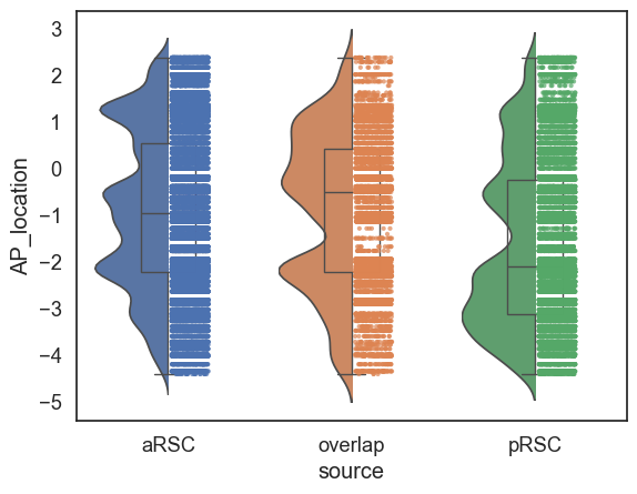
Plot the data with violin and box with dots
[3]:
df = load_example_rois()
_ = printdf(df, nrows=10)
shape: (45_163, 17)
┌─────────────────────────────────┬─────────┬─────────────┬─────────────┬─────────────┬─────────┬─────────┬────────┬───────────────────────────┬──────────────┬────────┬────────────┬────────────┬────────────┬────────────┬────────────┬───────────┐
│ name                            ┆ acronym ┆ AP_location ┆ DV_location ┆ ML_location ┆ avIndex ┆ channel ┆ source ┆ abbr                      ┆ acronym_abbr ┆ hemi.  ┆ merge_ac_0 ┆ merge_ac_1 ┆ merge_ac_2 ┆ merge_ac_3 ┆ merge_ac_4 ┆ family    │
│ ---                             ┆ ---     ┆ ---         ┆ ---         ┆ ---         ┆ ---     ┆ ---     ┆ ---    ┆ ---                       ┆ ---          ┆ ---    ┆ ---        ┆ ---        ┆ ---        ┆ ---        ┆ ---        ┆ ---       │
│ str                             ┆ str     ┆ f64         ┆ f64         ┆ f64         ┆ i64     ┆ str     ┆ str    ┆ str                       ┆ str          ┆ str    ┆ str        ┆ str        ┆ str        ┆ str        ┆ str        ┆ str       │
╞═════════════════════════════════╪═════════╪═════════════╪═════════════╪═════════════╪═════════╪═════════╪════════╪═══════════════════════════╪══════════════╪════════╪════════════╪════════════╪════════════╪════════════╪════════════╪═══════════╡
│ Ectorhinal area/Layer 5         ┆ ECT5    ┆ -3.03       ┆ 4.34        ┆ -4.5        ┆ 377     ┆ gfp     ┆ aRSC   ┆ Ectorhinal area           ┆ ECT          ┆ contra ┆ ECT        ┆ ECT        ┆ ECT        ┆ ECT        ┆ ECT        ┆ ISOCORTEX │
│ Perirhinal area layer 6a        ┆ PERI6a  ┆ -3.03       ┆ 4.42        ┆ -4.37       ┆ 372     ┆ gfp     ┆ aRSC   ┆ Perirhinal area           ┆ PERI         ┆ contra ┆ PERI       ┆ PERI       ┆ PERI       ┆ PERI       ┆ PERI       ┆ ISOCORTEX │
│ Perirhinal area layer 6a        ┆ PERI6a  ┆ -3.03       ┆ 4.55        ┆ -4.37       ┆ 372     ┆ gfp     ┆ aRSC   ┆ Perirhinal area           ┆ PERI         ┆ contra ┆ PERI       ┆ PERI       ┆ PERI       ┆ PERI       ┆ PERI       ┆ ISOCORTEX │
│ Perirhinal area layer 6a        ┆ PERI6a  ┆ -3.03       ┆ 4.5         ┆ -4.36       ┆ 372     ┆ gfp     ┆ aRSC   ┆ Perirhinal area           ┆ PERI         ┆ contra ┆ PERI       ┆ PERI       ┆ PERI       ┆ PERI       ┆ PERI       ┆ ISOCORTEX │
│ Entorhinal area lateral part l… ┆ ENTl5   ┆ -3.03       ┆ 4.92        ┆ -4.31       ┆ 504     ┆ gfp     ┆ aRSC   ┆ Entorhinal area           ┆ ENTl         ┆ contra ┆ HPF        ┆ RHP        ┆ ENT        ┆ ENT        ┆ ENTl       ┆ HPF       │
│ …                               ┆ …       ┆ …           ┆ …           ┆ …           ┆ …       ┆ …       ┆ …      ┆ …                         ┆ …            ┆ …      ┆ …          ┆ …          ┆ …          ┆ …          ┆ …          ┆ …         │
│ Temporal association areas lay… ┆ TEa6a   ┆ -2.91       ┆ 3.79        ┆ 4.45        ┆ 366     ┆ rfp     ┆ pRSC   ┆ Temporal association area ┆ TEa          ┆ ipsi   ┆ TEa        ┆ TEa        ┆ TEa        ┆ TEa        ┆ TEa        ┆ ISOCORTEX │
│ Ectorhinal area/Layer 6a        ┆ ECT6a   ┆ -2.91       ┆ 4.31        ┆ 4.45        ┆ 378     ┆ rfp     ┆ pRSC   ┆ Ectorhinal area           ┆ ECT          ┆ ipsi   ┆ ECT        ┆ ECT        ┆ ECT        ┆ ECT        ┆ ECT        ┆ ISOCORTEX │
│ Ventral auditory area layer 6a  ┆ AUDv6a  ┆ -2.91       ┆ 3.52        ┆ 4.46        ┆ 156     ┆ rfp     ┆ pRSC   ┆ Ventral auditory area     ┆ AUDv         ┆ ipsi   ┆ AUD        ┆ AUD        ┆ AUD        ┆ AUD        ┆ AUDv       ┆ ISOCORTEX │
│ Ectorhinal area/Layer 6a        ┆ ECT6a   ┆ -2.91       ┆ 4.14        ┆ 4.47        ┆ 378     ┆ rfp     ┆ pRSC   ┆ Ectorhinal area           ┆ ECT          ┆ ipsi   ┆ ECT        ┆ ECT        ┆ ECT        ┆ ECT        ┆ ECT        ┆ ISOCORTEX │
│ Temporal association areas lay… ┆ TEa5    ┆ -2.91       ┆ 4.02        ┆ 4.55        ┆ 365     ┆ rfp     ┆ pRSC   ┆ Temporal association area ┆ TEa          ┆ ipsi   ┆ TEa        ┆ TEa        ┆ TEa        ┆ TEa        ┆ TEa        ┆ ISOCORTEX │
└─────────────────────────────────┴─────────┴─────────────┴─────────────┴─────────────┴─────────┴─────────┴────────┴───────────────────────────┴──────────────┴────────┴────────────┴────────────┴────────────┴────────────┴────────────┴───────────┘
[4]:
sns.set(style='white', font_scale=1.2)
fig, ax = plt.subplots()
violin_boxplot(data=df, x='source', y='AP_location', hue='source', ax=ax)
plt.show()
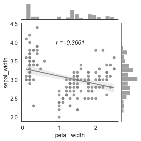
See correlation and histogram of two variables
[5]:
iris = sns.load_dataset('iris')
x = iris['petal_width']
y = iris['sepal_width']
scatter_histogram(x, y, linear_reg=True, bins=20)
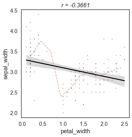
See y as a function of x
dotted line indicates the binned median or mean y values
[6]:
_, ax = plt.subplots()
scatter_binx_plot(ax=ax, x=x, y=y, bins=10, bin_func='median')
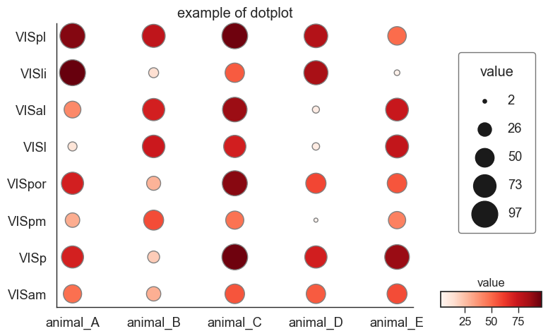
Dotsplot with colormap
[7]:
# (X,): different animals
xlabel = ['animal_A', 'animal_B', 'animal_C', 'animal_D', 'animal_E']

# (Y,): subregion in Visual Cortex as an example
ylabel = ['VISam', 'VISp', 'VISpm', 'VISpor', 'VISl', 'VISal', 'VISli', 'VISpl']

# values: Array[float, [X, Y]]
nx = len(xlabel)
ny = len(ylabel)
values = np.random.sample((nx, ny)) * 100

dotplot(xlabel, ylabel, values,
        scale='area',
        max_marker_size=700,
        with_color=True,
        figure_title='example of dotplot')
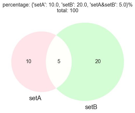
Venn Diagram
[8]:
# 2 sets
subsets = {'setA': 10, 'setB': 20}
vd = VennDiagram(subsets, colors=('pink', 'palegreen'))
vd.add_intersection('setA & setB', 5)
vd.add_total(100)
vd.plot()
vd.show()
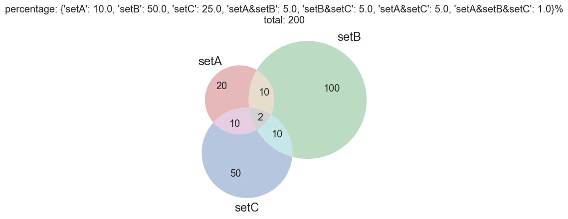
[9]:
# 3 sets
subsets = {'setA': 20, 'setB': 100, 'setC': 50}
vd = VennDiagram(subsets)
vd.add_intersection('setA & setB', 10)
vd.add_intersection('setB & setC', 10)
vd.add_intersection('setA & setC', 10)
vd.add_intersection('setA & setB & setC', 2)
vd.add_total(200)
vd.plot()
vd.show()
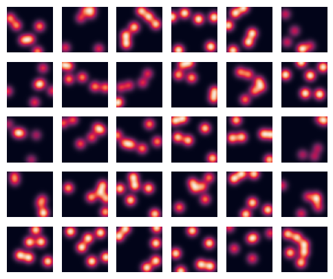
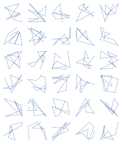
Grid subplots
[10]:
data = np.random.sample((30, 10, 2))
grid_subplots(data, 5, 'plot', dtype='xy', ls='dotted')
[11]:
def generate_example_2d_tuning(blobs: int = 6) -> np.ndarray:
    """example mimic place cell place cell firing"""
    x, y = np.meshgrid(np.linspace(0, 6, 50), np.linspace(0, 6, 50))
    z = np.zeros_like(x)

    for _ in range(blobs):
        x0 = np.random.uniform(0, 6)
        y0 = np.random.uniform(0, 6)
        sigma = 0.5
        z += np.exp(-((x - x0) ** 2 + (y - y0) ** 2) / (2 * sigma ** 2))

    return z


data = [generate_example_2d_tuning() for i in range(30)]
grid_subplots(data, images_per_row=6, plot_func='imshow', dtype='img')