Example notebook neuralib.model.rastermap

• See also the reference GitHub rastermap

  • cellular example

  • widefield example

import numpy as np

from neuralib.imglib.io import load_sequence
from neuralib.io.dataset import load_example_rastermap_2p_cache
from neuralib.model.rastermap import (
    Covariant,
    run_rastermap,
    plot_rastermap,
    plot_cellular_spatial,
    plot_wfield_spatial,
    RasterOptions
)

%load_ext autoreload
%autoreload

The autoreload extension is already loaded. To reload it, use:
  %reload_ext autoreload

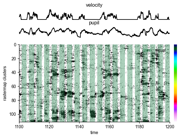
Example of cellular dataset

• Two-photon imaging during linear treadmill

• Tracking of behavioral variables. velocity, pupil area

# download cache, replace your own neural activity array
cache = load_example_rastermap_2p_cache(cached=True, rename_file='raster_2p')
result = run_rastermap(cache['neural_activity'], bin_size=10, dtype='cellular')

2025-12-19 11:19:25,796 [INFO] normalizing data across axis=1
2025-12-19 11:19:26,184 [INFO] projecting out mean along axis=0
2025-12-19 11:19:26,489 [INFO] data normalized, 0.69sec
2025-12-19 11:19:26,491 [INFO] sorting activity: 1118 valid samples by 108128 timepoints
2025-12-19 11:19:30,572 [INFO] n_PCs = 128 computed, 4.78sec
2025-12-19 11:19:30,856 [INFO] 31 clusters computed, time 5.06sec
2025-12-19 11:19:31,196 [INFO] clusters sorted, time 5.40sec
2025-12-19 11:19:31,254 [INFO] clusters upsampled, time 5.46sec
2025-12-19 11:19:31,662 [INFO] rastermap complete, time 5.87sec

# plot map together with behavioral measurement (running velocity and pupil size)
# In example, interpolated time has same shape between covariant and activity, but non-interpolated time is also supported
time = cache['image_time']
vel = Covariant('velocity', dtype='continuous', time=time, value=cache['velocity'])
pupil = Covariant('pupil', dtype='continuous', time=time, value=cache['pupil_area'])
visual_event = Covariant('visual', dtype='event', time=cache['visual_stim_time'], value=None)
plot_rastermap(result, time, time_range=(1100, 1200), covars=[vel, pupil, visual_event])

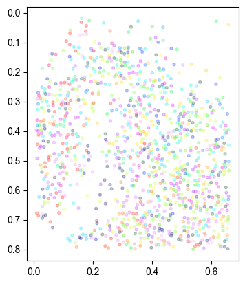
# plot the neuron location with color-coded
xy_pos = cache['xy_pos']
plot_cellular_spatial(result, xy_pos[0], xy_pos[1])

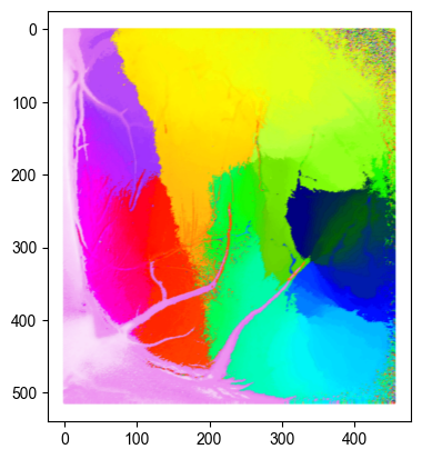
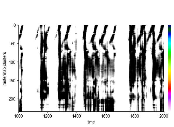
Example of widefield imaging dataset

• Wide-field imaging for retinotopic mapping using circular patch visual stimuli

# load sequence neural activity from path OR an array with `Array[Any, [T, H, W]]`
tiff_path = ...
neural_activity = load_sequence(tiff_path)
nframe, height, width = neural_activity.shape

opt: RasterOptions = {
    'n_clusters': 30,
    'n_PCs': 128,
    'locality': 0.5,
    'time_lag_window': 10,
    'grid_upsample': 10
}
result = run_rastermap(neural_activity,
                       bin_size=1000,
                       dtype='wfield',
                       options=opt,
                       svd_components=128,
                       svd_cache=...)  # local pkl cache for svd compute

Loading TIFF sequence: 100%|██████████| 1/1 [00:00<00:00, 273.96file/s]

2025-04-22 21:54:08,099 [INFO] data normalized, 0.06sec
2025-04-22 21:54:08,106 [INFO] sorting activity: 234840 valid samples by 2816 timepoints
2025-04-22 21:54:24,384 [INFO] 30 clusters computed, time 16.34sec
2025-04-22 21:54:24,569 [INFO] clusters sorted, time 16.53sec
2025-04-22 21:54:25,171 [INFO] clusters upsampled, time 17.13sec
2025-04-22 21:54:25,193 [INFO] rastermap complete, time 17.15sec

# plot rastermap
plot_rastermap(result, np.arange(result.n_samples), time_range=(1000, 2000))

# plot the spatial location across xy pixel
plot_wfield_spatial(result, width, height)