neuralib.atlas.brainrender
BrainRender Wrapper
- author:
Yu-Ting Wei
This module provides a CLI-based wrapper for brainrender. Once installed, the CLI can be invoked directly from the command line.
To see available options, use the -h flag:
neuralib_brainrender {area, roi, probe} -h
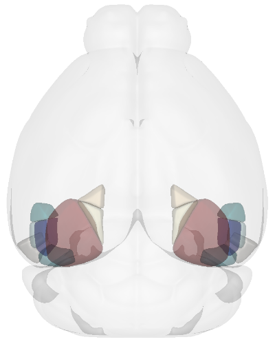
Region Reconstruction
Example: Reconstructing the Visual Cortex from specified brain regions:
neuralib_brainrender area -R VISal,VISam,VISl,VISli,VISp,VISpl,VISpm,VISpor --camera top
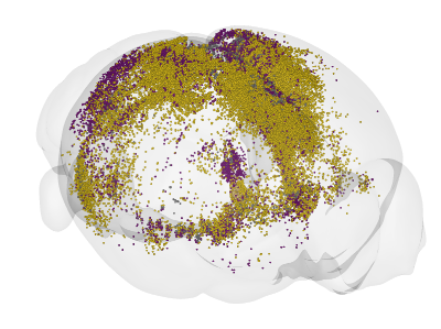
ROI Reconstruction
By default, coordinates are interpreted in the CCF coordinate space.
You can specify the coordinate space using the --coord-space option: {ccf, brainrender}.
NumPy File Input
Input shape: Array[float, (N, 3)], with AP, DV, and ML coordinates.
Example:
[[-3.03,  4.34, -4.50],
 [-3.03,  4.42, -4.37],
 ...
 [-2.91,  4.12,  4.85]]
Run:
neuralib_brainrender roi --file <NUMPY_FILE>
CSV File Input
Required columns: AP_location, DV_location, ML_location
┌─────────────┬─────────────┬─────────────┐
│ AP_location │ DV_location │ ML_location │
│------------ │-------------│-------------│
│ -3.03       │ 4.34        │ -4.50       │
│ -3.03       │ 4.92        │ -4.31       │
│ ...         │ ...         │ ...         │
│ -2.91       │ 4.12        │ 4.85        │
└─────────────┴─────────────┴─────────────┘
Example:
neuralib_brainrender roi --file <CSV_FILE>
Flexible Reconstruction (Processed CSV)
Be able to reconstruct rois in a specific regions/subregions
Example of using parsed allenccf csv output
┌───────────────────────────────────┬─────────┬─────────────┬─────────────┬─────────────┬─────────┬─────────┬────────┬────────────┐
│ name                              ┆ acronym ┆ AP_location ┆ DV_location ┆ ML_location ┆ avIndex ┆ channel ┆ source ┆  ...       │
│ ---                               ┆ ---     ┆ ---         ┆ ---         ┆ ---         ┆ ---     ┆ ---     ┆ ---    ┆  ---       │
│ str                               ┆ str     ┆ f64         ┆ f64         ┆ f64         ┆ i64     ┆ str     ┆ str    ┆  ...       │
╞═══════════════════════════════════╪═════════╪═════════════╪═════════════╪═════════════╪═════════╪═════════╪════════╪════════════╡
│ Ectorhinal area/Layer 5           ┆ ECT5    ┆ -3.03       ┆ 4.34        ┆ -4.5        ┆ 377     ┆ gfp     ┆ VIS    ┆  ...       │
│ Perirhinal area layer 6a          ┆ PERI6a  ┆ -3.03       ┆ 4.42        ┆ -4.37       ┆ 372     ┆ gfp     ┆ VIS    ┆  ...       │
│ …                                 ┆ …       ┆ …           ┆ …           ┆ …           ┆ …       ┆ …       ┆ …      ┆  …         │
│ Ventral auditory area layer 6a    ┆ AUDv6a  ┆ -2.91       ┆ 3.52        ┆ 4.46        ┆ 156     ┆ rfp     ┆ CA1    ┆  ...       │
│ Ectorhinal area/Layer 6a          ┆ ECT6a   ┆ -2.91       ┆ 4.14        ┆ 4.47        ┆ 378     ┆ rfp     ┆ CA1    ┆  ...       │
│ Temporal association areas layer… ┆ TEa5    ┆ -2.91       ┆ 4.02        ┆ 4.55        ┆ 365     ┆ rfp     ┆ CA1    ┆  ...       │
└───────────────────────────────────┴─────────┴─────────────┴─────────────┴─────────────┴─────────┴─────────┴────────┴────────────┘
import polars as pl
from neuralib.atlas.ccf.classifier import RoiClassifierDataFrame

df = pl.DataFrame({
    "acronym": ["RSPd", "RSPd", "VISp", "VISp"],
    "AP_location": [1.2, 1.3, -2.4, -2.6],
    "DV_location": [1.0, 1.1, 2.0, 2.1],
    "ML_location": [0.4, -0.3, 0.2, -0.2],
    "channel": ["gfp", "gfp", "rfp", "rfp"],
    "source": ["CA1", "CA1", "CA3", "CA3"]
})

df = RoiClassifierDataFrame(df).post_processing().dataframe()
df.write_csv(CSV_FILE)
See also
Example (reconstruct ROI in the parahippocampal areas):
neuralib_brainrender roi --classifier-file <CSV_FILE> --region APr,ENT,HATA,PAR,POST,PRE,ProS,SUB --roi-region RHP --region-alpha 0.2 --roi-radius 20 --no-root -H right

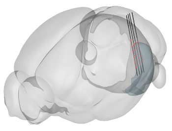
Probe Reconstruction
Reconstruct probes (or shanks) based on trajectory labeling (e.g., DiI, DiO, or lesion tracks).
Default coordinate space: CCF
Set coordinate space using:
--coord-space {ccf, brainrender}Each shank must have 2 points: dorsal and ventral
NumPy File Input
Single shank: Array[float, (2, 3)] (dorsal and ventral 3D AP/ML/DV coordinates)
[[-3.82, 1.92, -3.12],
 [-3.93, 4.36, -3.30]]
Multi-shank: Array[float, (S, 2, 3)]
[[[...], [...]],
 [[...], [...]],
 ...]
CSV File Input
Required fields: AP_location, DV_location, ML_location, point, probe_idx
If loss either point, probe_idx field, then auto infer based on the given insertion --plane
┌─────────────┬─────────────┬─────────────┬─────────┬───────────┐
│ AP_location │ DV_location │ ML_location │ point   │ probe_idx │
├─────────────┼─────────────┼─────────────┼─────────┼───────────┤
│ -3.81       │ 1.92        │ -3.12       │ dorsal  │ 1         │
│ -3.93       │ 4.36        │ -3.30       │ ventral │ 1         │
│ ...         │ ...         │ ...         │ ...     │ ...       │
└─────────────┴─────────────┴─────────────┴─────────┴───────────┘
Additional Options
--depth DEPTH: Depth (in µm) of the implantation from the brain surface--dye: Only reconstruct dye-labeled tracks (default includes both dye and theoretical)--remove-outside-brain: Exclude any segments outside the brain
Example: Reconstructing a 4-shank NeuroPixel probe targeting the left entorhinal cortex
neuralib_brainrender probe -F <FILE> --depth 3000 -P sagittal -R ENT -H left
Red = dye-labeled track
Black = theoretical track
Help
To explore available options for each subcommand, use the -h flag:
neuralib_brainrender probe -h